Every blockchain has some state associated with it. That state can be thought of as a collection of key/value pairs. This state might represent something simple, like how many tokens each account has. The state might represent something more complicated like the code of a smart contract. No matter what this state represents, everyone on the blockchain has to reach agreement. If I thought that you had ten tokens, but you thought that you had a million tokens, we obviously couldn’t get much done until we figured out which of us was right.

Unfortunately reaching agreement about the state is quite a big problem. One issue is how to set things up so that bad participants can never trick trustworthy participants into accepting a bad state. The other issue is that the state is very large. How can participants reach agreement quickly if even transmitting the state takes a long time? In this article we will talk about one possible solution to the latter issue, the Merkle trie.

What is a Merkle Trie?

A Merkle trie is a data structure that combines the features of two other data structures. The first is a Merkle tree and the second is a radix trie.

What is a Merkle Tree?

A Merkle tree is a special type of tree. The special feature of Merkle trees is that they generate “fingerprints” for each part of the tree, as well as the whole tree. Just like a real fingerprint, the ones generated by the tree are fairly unique. Whenever you change any data in the tree, the fingerprint changes as well.

This provides us with a solution to the problem of communicating what each participant thinks the state currently is. You can take the fingerprint that represents the entire tree and send it to other blockchain participants. If everyone has generated the same fingerprint for the state data, then they must have the same state. If the fingerprints are different then the state must have been different.

What is a Radix Trie?

A radix trie is a special type of trie (a trie is a special type of tree) that makes storing and retrieving key/value pairs easy. A Merkle tree is really good at allowing you to prove that some data is part of the tree, but it does not make it easy to look up the values associated with keys, so we combine the radix trie and the Merkle tree to get something that can do both.

How does it all work?

The exact details of how a Merkle trie works can vary as there are many different ways to implement similar functionality. Trying to explain all of these different ways is beyond the scope of this article, so the rest of this article will describe just one particular implementation.

It’s nodes all the way down

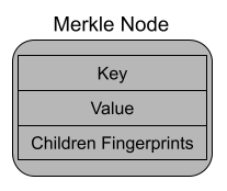
The Merkle trie is made up of just one object, nodes. Each node is a little chunk of data that is stored within the trie. The data each node contains is key information, value information (if one exists for the node’s key), and the fingerprints of any children nodes.

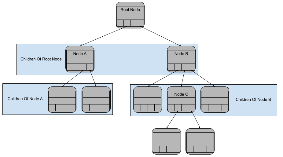
The nodes directly “under” a node are called children nodes. The node “above” a node is called the parent node. Each node has just one parent, but can have many children. There is one special node in the trie that has no parent. This is the node at the “top” of the trie and it is called the root node.

Generating fingerprints

How do you use a Merkle trie to generate the fingerprint of each node? The most common way is to use a cryptographic hash function. A lot of different cryptographic hash functions exist, but they all share two features important to Merkle tries.

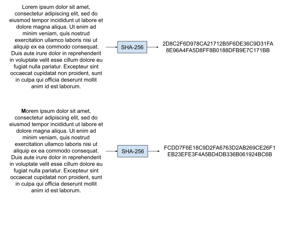
The first feature of a hash function is that it takes in data as input and outputs a number of fixed size that represents that data. Usually the number that is output is significantly smaller in size than the input data. For example, SHA-256, a popular hash function, takes inputs of any size and generates an output number 256 bits long. The function is very sensitive, so small changes in the input will lead to large differences in the output.

The number that the hash function outputs is the fingerprint that we want. For each node, we apply the hash function to the data in the node and use the generated number as the node’s fingerprint. The fingerprints of the node’s children are part of a node’s data, so the fingerprint for a node also covers all of the data in the trie that is under the node. We can now represent all of the data in the trie with the fingerprint of the root node.

The second feature of hash functions is that it needs to be very difficult to “reverse” the function, i.e. given some output number, find any inputs that would generate that number. If the hash function were easy to reverse, someone could find different state data that generated the same number. They could use this to trick other participants and cause problems. Luckily, this is not easy to do, which allows blockchain participants to trust that if they generated the same fingerprint as other participants, they have the same data.

One issue with cryptographic hash functions is that they tend to be somewhat slow to calculate. On one hand, this slowness is a security feature. If you wanted to create a fake state with the same hash function output, you could repeatedly try different inputs until you found something that worked. The slower it is to execute the hash function, the longer that search will take. On the other hand, slow calculation speed can make using the Merkle trie slower since it makes a lot of calls to the hash function in normal usage.

Finding a key/value pair

Recall that the data in this Merkle trie is the current blockchain state and that the state is made up of key/value pairs. One of the common actions that you have to do is look up the value associated with a key. This is done by turning the key into a path through the trie. By starting at the Root node and then following this key path, you will end up at the node that stores the value you want.

Turning the key into a path

Somehow we need to go from a key to a set of steps to take through the trie. So we need to break the key up into smaller parts and each part will determine our next step. To make this process easier, let’s represent keys as binary data (a number made up of just 0 and 1). This makes it easy to break up the key into smaller chunks and then convert the chunks into numbers. These numbers tell us which node to visit next.

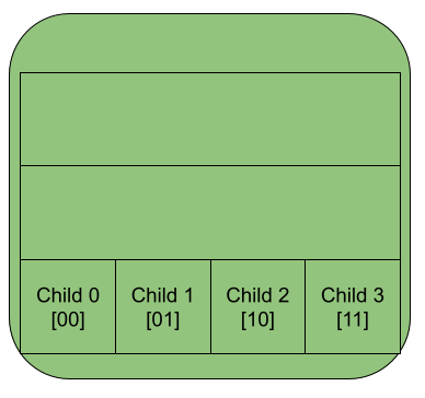
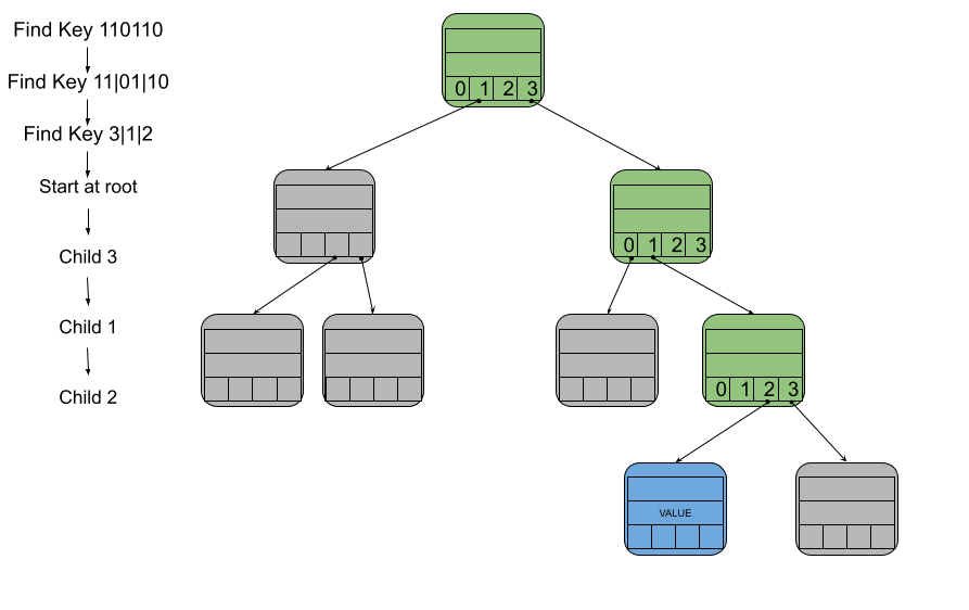
In this implementation, let us limit each node to having at most 4 children. If we split up the key into pairs of bits, then each pair will tell us which of the 4 children to visit next. This correspondence between bits and child nodes is possible because there are the same number of both. The 4 different possible pairs of bits [00, 01, 10, 11] correspond to the 4 different child nodes [0, 1, 2, 3].

For example, in the diagram below, you have key 110110. First you would break it up into pairs 11|01|10. Turning those into child numbers would be 3|1|2. All paths start at the root node, so to follow the path to the node with key 110110 we begin at the root node. Then you would move to child 3 of the root. Then you would move to child 1 of that node. Finally you would move to child 2 of that node. That last node that would then contain the value for key 110110.

Compressing the path

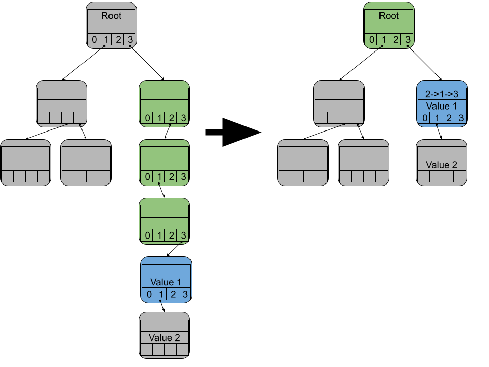
If you construct the key path exactly as described above, you end up creating a lot of empty nodes. These empty nodes are created because every pair of bits corresponds to a node. If the key had 1000 bit pairs, the path would have 1000 nodes in it. This slows down the search since each of the 1000 nodes would be visited before finding the node with the value we wanted.

To prevent searches from being slow, we can compress the extra nodes into a single node. For each node that gets compressed, we record which child number it was. Then we put that list of numbers into the combined node. While traveling along a key path, if the current node has a compressed path that matches the current key, you can skip ahead.

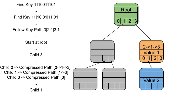
With compressed paths in the mix, searching changes a little. If you come across a node with a compressed path during a search, then for each remaining step in the key path, check if it matches the next step from the compressed path. If they match, then move onto the next step in the key path and the compressed path. If they don’t then the key you were looking for wasn’t in the trie.

For example, let’s say you have been traveling along a key path and the node we have reached has a compressed path of [3->2] and the remaining steps of the key path are [child 3 -> child 2 -> child 0]. In this scenario, the next step of the key path is [child 3] and the next step of the compressed path is [child 3]. These match, so we move onto the next step. The next step from the key path is [child 2] and the next step of the compressed path is [child 2], these match so again we move onto the next step. The next step of the key path is [child 0] and the compressed path has no more steps, so we go to child 0 of the current node and we are done.

Inserting a key/value pair

Inserting a key/value pair into the trie is very similar to searching for an existing key. The main difference is the key you are looking for might not be in the trie. While following the key path, one of several situations will occur. You will either find the node that corresponds to that key, run out of nodes to search, or you hit a node that has a compressed path that does not match the key path.

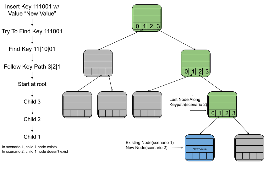
• Scenario 1: Find a node corresponding to the key
  If there is a node with the key in the trie, then it will be at the end of the key path. Once we have found that node, simply add the new value to it.
• Scenario 2: Ran out of nodes while following the key path
  When there is no node that corresponds to the key, we will get to a step in the key path that we can’t take since no node exists. In this case, we simply create a new node and add it as a child of that last node that did exist along the key path.

• Scenario 3: Conflicting Compressed Path Found
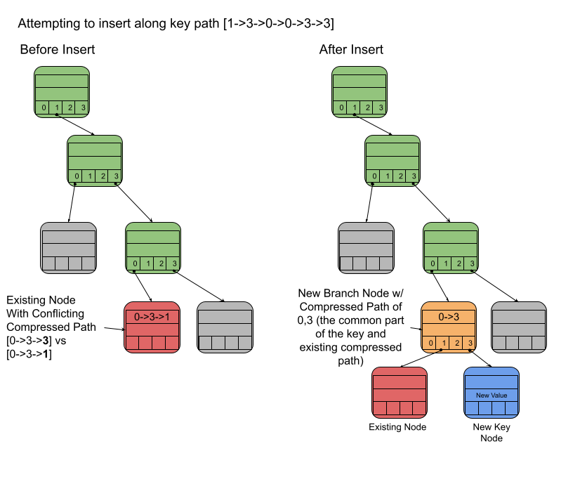
  While traversing the key path, you may hit a node that has a compressed path that does not match the key being inserted. This means that a new node that can allow the path to “branch” needs to be inserted along with the new key/value pair node. The entire process follows these steps:

​ ​ ​​​ ​ ​​​ ​ ​​​ ​ ​​​ ​ ​​1. Create a new “Branch” node. Its compressed path will be equal to ​ ​ ​​​ ​ ​​​ ​ ​​​ ​ ​​​ ​ ​​​ ​ ​​​ ​ ​​​ ​ ​​​ ​ ​​​ ​ ​​any common path steps between the new key path and the existing ​ ​ ​​​ ​ ​​​ ​ ​​​ ​ ​​​ ​ ​​​ ​ ​​​ ​ ​​​ ​ ​​node’s compressed path.

​ ​ ​​​ ​ ​​​ ​ ​​​ ​ ​​​ ​ ​​2. Move the existing node to be a child of the “Branch” node

​ ​ ​​​ ​ ​​​ ​ ​​​ ​ ​​​ ​ ​​3. Create a new node for the key/value pair and add that as a child of ​ ​ ​​​ ​ ​​​ ​ ​​​ ​ ​​​ ​ ​​​ ​ ​​​ ​ ​​​ ​ ​​​ ​ ​​​ the “Branch” node

Sharing the state

When someone joins the blockchain for the first time, they don’t have any of the blockchain’s state. Without that state, they won’t be able to interpret and verify the transactions that occur. One way to get the state is to start at the very beginning of the blockchain and then play through every transaction that has ever occurred. If the blockchain has existed for a while, this might take a really long time.

An alternative is to request the state from other blockchain participants. Unfortunately in a blockchain, you cannot trust the other participants. The Merkle trie helps solve this trust problem as well. The Merkle trie can be used to “prove” that a key/value pair is in it. By sending along a proof for the key/value, it is possible to be sure that the data is accurate and trustworthy.

Proving the value of a Single Key

Given a Merkle Trie, a proof that a given key/value pair is in the trie can be formed by providing all of the data in the nodes along its key path.

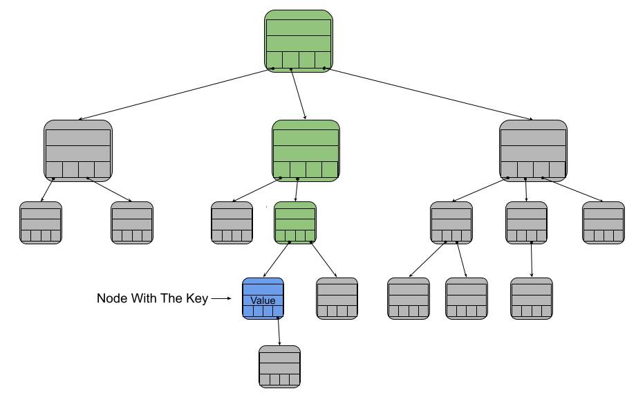
The data from these nodes act as a proof of the blue node’s value. To verify the proof, you insert all of that data into an empty trie. That trie’s root will have some fingerprint. If that fingerprint matches the one that all of the blockchain participants have agreed upon, then the proof is considered verified. It is very difficult to generate fake data that will produce the same fingerprint, so this proof allows us to be confident that the key/value pair that was sent really is part of the blockchain’s state.

Proving values for a Range of Keys

We need to get all of the state data, but it would be inefficient to have to generate and send a proof for every pair. Instead, we can extend the proof concept to a proving a range of key/value pairs.

This range proof consists of three parts. The first is the proof of a starting key, the second is a proof of the ending key. These work just as described above, by sending all the nodes on the path to finding the starting and ending keys. The third and final part is all of the key/value pairs that fall between the start and end. Since only the key/value pairs are sent for the nodes between the state and end, this proof is much smaller than constructing proofs for each key/value pair individually. This reduced size allows for more efficient transmission of the data within the trie.

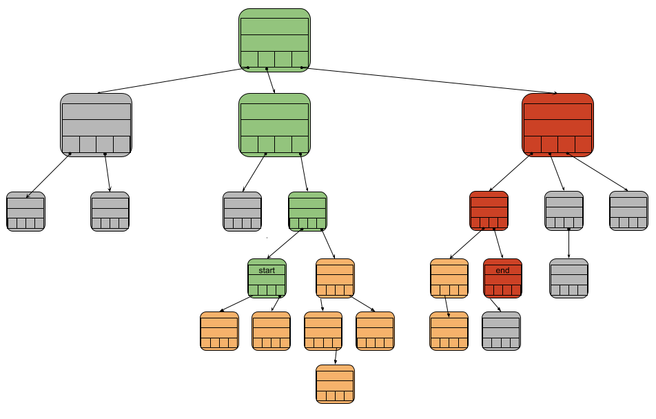
Similar to the verification of the single key/value pair proof, the data from the start proof nodes, end proof nodes, and all of the key/value pairs can be inserted into an empty trie. If the fingerprint of the root node of this trie matches the agreed upon fingerprint, then all of the key/value pairs sent in the proof are considered valid state data.

Conclusion

With a Merkle trie you can insert/retrieve key/values pairs, reach agreement about the blockchain’s state, and share proofs of the state with other participants. These features cover a large portion of the functionality required to run a trustless blockchain. This is still an active area of research though, so maybe you can come up with something even better!

Where to go from here?

If you are still curious, there are a lot of options for further reading. If you are code inclined, a go implementation of a Merkle Trie similar to the one described above can be viewed here. If you are curious about other implementations of Merkle tries, check out this wiki entry on Ethereum’s Merkle implementation. If you are more academically inclined, this paper on polynomial commitments provides an interesting alternative for generating the node fingerprints and proofs of the blockchain state.

---

From the Labs: Handling Blockchain State was originally published in Avalanche on Medium, where people are continuing the conversation by highlighting and responding to this story.

Source